Control Systems Engineering

Citation

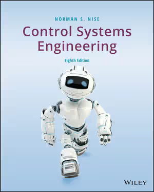
Nise, N. S. (2019). Control Systems Engineering (8th ed.). Wiley.

Chapter Summary

The book runs to about 800 pages in thirteen chapters. Each chapter opens with learning outcomes, closes with a summary, review questions and a bibliography, and most include case studies, and each ends with a "Cyber Exploration Laboratory" of software experiments. A running case study, an antenna azimuth position control system, is carried through the chapters and is described in an appendix.

Chapter 1: Introduction

Defines a control system, lists the reasons for building one (power amplification, remote control, convenience of input form, compensation for disturbances) and introduces the two basic performance measures, transient response and steady-state error. The chapter also gives a short history, system configurations, the analysis and design objectives, the design process and the role of computer-aided design.

Chapter 2: Modeling in the Frequency Domain

Reviews the Laplace transform and defines the transfer function, then derives transfer functions for electrical networks, translational and rotational mechanical systems, systems with gears and electromechanical systems. It closes with electric circuit analogs, nonlinearities and linearization.

Chapter 3: Modeling in the Time Domain

The state-space counterpart of Chapter 2: the general state-space representation, its application to physical systems, conversion between a transfer function and state space, and linearization.

Chapter 4: Time Response

Uses the poles and zeros of a transfer function to predict response. It covers first-order systems, second-order systems (introduced, then treated in general and in the underdamped case), the effect of additional poles and of zeros, the effect of nonlinearities, and the solution of state equations in the Laplace and time domains.

Chapter 5: Reduction of Multiple Subsystems

Shows how to combine subsystems into one model, with block diagrams, signal-flow graphs and Mason's rule. It also treats signal-flow graphs of state equations, alternative state-space representations and similarity transformations.

Chapter 6: Stability

Presents the Routh-Hurwitz criterion, its special cases and further examples, then stability in state space.

Chapter 7: Steady-State Errors

Covers steady-state error for unity-feedback systems, static error constants and system type, error specifications, error for disturbances and for nonunity-feedback systems, sensitivity, and steady-state error for systems in state space.

Chapter 8: Root Locus Techniques

Defines the root locus, its properties and the steps for sketching and refining it, then uses it for transient response design by gain adjustment. Further sections cover the generalized root locus, positive-feedback systems and pole sensitivity.

Chapter 9: Design via Root Locus

Uses cascade compensation on the root locus to improve steady-state error, transient response or both, then treats feedback compensation and the physical realization of compensators.

Chapter 10: Frequency Response Techniques

Introduces Bode plots through asymptotic approximations and the Nyquist criterion, including sketching the diagram, stability, and gain and phase margin. Later sections relate open-loop and closed-loop frequency response to transient response and steady-state error, and cover systems with time delay and the experimental determination of transfer functions.

Chapter 11: Design via Frequency Response

Designs compensators in the frequency domain: transient response via gain adjustment, then lag, lead and lag-lead compensation.

Chapter 12: Design via State Space

Covers controller design, controllability, alternative controller design approaches, observer design, observability and alternative observer designs, and steady-state error design via integral control.

Chapter 13: Digital Control Systems

Models the digital computer in the loop and introduces the z-transform and discrete transfer functions. It then adapts block-diagram reduction, stability, steady-state error, transient response and gain design to the z-plane, and ends with cascade compensation via the s-plane and implementation of the digital compensator.

Key Concepts

Chapters 1–3: Introduction and modeling

• Transient response and steady-state error: the two performance measures that frame all later analysis and design.
• Transfer function: the frequency-domain input-output description of a linear system, built for electrical, mechanical and electromechanical components.
• State-space representation: a time-domain model that also handles multiple inputs and outputs.
• Linearization: approximating a nonlinear system by a linear one near an operating point.

Chapters 4–7: Analysis

• Poles and zeros: their locations determine the form of the response.
• Routh-Hurwitz criterion: a test of stability from the characteristic polynomial.
• System type and static error constants: the way steady-state error is predicted for standard inputs.

Chapters 8–11: Classical design

• Root locus: the paths of the closed-loop poles as gain varies.
• Bode and Nyquist methods: frequency-response tools for stability, gain margin and phase margin.
• Lag, lead and lag-lead compensation: cascade compensators used to improve steady-state error and transient response.

Chapters 12–13: State-space and digital design

• Controllability and observability: conditions under which state feedback and state estimation are possible.
• Observer design: estimating states that are not measured.
• z-transform: the discrete-time counterpart of the Laplace transform used for computer-controlled systems.

Critical Analysis

Strengths

• Design emphasis throughout. The publisher describes the book as going beyond theory and abstract mathematics to translate concepts into physical control system design, with step-by-step procedures. The contents bear this out: Chapters 9, 11 and 12 are devoted to design in the three main domains.
• Case studies and a running example. Chapters carry case studies, and the antenna azimuth position control system is followed from chapter to chapter, which lets a reader see one system analysed with each new technique.
• Software and hardware practice. Every chapter ends with a Cyber Exploration Laboratory, several chapters with a Hardware Interface Laboratory, and the appendices give tutorials for MATLAB, Simulink, LabVIEW and related tools.
• Self-study aids. Every chapter has review questions and fully worked practice problems accompany the updated end-of-chapter problems (the publisher notes these as new in the eighth edition); answers to selected problems and a glossary are included.

Limitations

• A long, wide book. At about 800 pages it covers both classical and modern control, so a one-semester course must select; the state-space and digital chapters come after the classical-design chapters and may not fit in a first course.
• Software-dependent parts. The laboratory exercises and several appendices assume access to MATLAB, Simulink or LabVIEW, and some appendices are available only in the e-text.
• Procedure-oriented. The book emphasizes step-by-step methods and applications over abstract mathematics, as the publisher's description says; readers who want a more theoretical treatment of control will need a second text.

Where It Fits in the Course

Nise is the main applied text in this course list for a first course on feedback control. Oppenheim and Willsky's Signals and Systems covers the Laplace and z-transforms and ends with an introduction to feedback; it is a sensible preparation for Nise's Chapters 2 and 13, while Sadiku's primer and Downey's Think DSP are lighter, example-driven routes to the same transform ideas.

Åström and Murray's Feedback Systems is a modern introduction that extends feedback ideas to biological and information systems and stresses modeling, state space and robustness; it pairs well with Nise as a second perspective after the classical techniques. Craig's Introduction to Robotics applies control to robot arms and assumes a background in control, so it is best read after Nise's Chapters 1–10.

How to Use This Book

The book suits second- or third-year engineering students who have met differential equations, Laplace transforms, linear algebra and basic dynamics or circuits. The publisher positions it for core control courses in mechanical, electrical, aerospace, biomedical and chemical engineering.

A practical plan for a first course:

• Core: Chapters 1–10 in order. Chapters 2, 4, 6 and 7 build the modeling, response, stability and error vocabulary that every later design chapter assumes.
• Design: read Chapter 8 before Chapter 9, and Chapter 10 before Chapter 11, so the analysis technique is understood before it is used for compensation.
• Later or optional: Chapters 3 and 5 (the state-space parts), 12 and 13. Read Chapter 3 earlier if the course is state-space oriented.

Work the review questions first, then the practice problems, then the end-of-chapter problems. Repeat the case study for each chapter on a computer, using the Cyber Exploration Laboratory sections, and compare the software result with the hand sketch of the root locus or Bode plot.